Adapter Methods
On this page, we present all adapter methods currently integrated into the adapters library.
A tabular overview of adapter methods is provided here.
Additionally, options to combine multiple adapter methods in a single setup are presented on the next page.
Bottleneck Adapters
Configuration class: BnConfig
Bottleneck adapters introduce bottleneck feed-forward layers in each layer of a Transformer model. Generally, these adapter layers consist of a down-projection matrix \(W_{down}\) that projects the layer hidden states into a lower dimension \(d_{bottleneck}\), a non-linearity \(f\), an up-projection \(W_{up}\) that projects back into the original hidden layer dimension and a residual connection \(r\):
Depending on the concrete adapter configuration, these layers can be introduced at different locations within a Transformer block. Further, residual connections, layer norms, activation functions and bottleneck sizes ,etc., can be configured.
The most important configuration hyperparameter to be highlighted here is the bottleneck dimension \(d_{bottleneck}\).
In adapters, this bottleneck dimension is specified indirectly via the reduction_factor attribute of a configuration.
This reduction_factor defines the ratio between a model’s layer hidden dimension and the bottleneck dimension, i.e.:
A visualization of further configuration options related to the adapter structure is given in the figure below. For more details, we refer to the documentation of BnConfig](adapters.BnConfig).
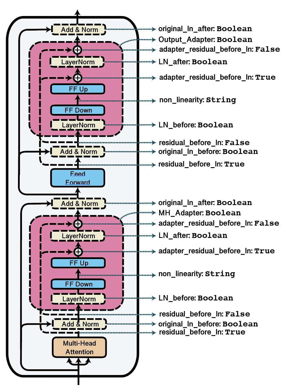
Visualization of possible adapter configurations with corresponding dictionary keys.
adapters comes with pre-defined configurations for some bottleneck adapter architectures proposed in literature:
DoubleSeqBnConfig, as proposed by Houlsby et al. (2019) places adapter layers after both the multi-head attention and feed-forward block in each Transformer layer.SeqBnConfig, as proposed by Pfeiffer et al. (2020) places an adapter layer only after the feed-forward block in each Transformer layer.ParBnConfig, as proposed by He et al. (2021) places adapter layers in parallel to the original Transformer layers.AdapterPlusConfig, as proposed by Steitz and Roth (2024) places adapter layers adapter layers after the multi-head attention and has channel wise scaling and houlsby weight initialization Example:
from adapters import BnConfig

config = BnConfig(mh_adapter=True, output_adapter=True, reduction_factor=16, non_linearity="relu")
model.add_adapter("bottleneck_adapter", config=config)
Papers:
Parameter-Efficient Transfer Learning for NLP (Houlsby et al., 2019)
Simple, Scalable Adaptation for Neural Machine Translation (Bapna and Firat, 2019)
AdapterFusion: Non-Destructive Task Composition for Transfer Learning (Pfeiffer et al., 2021)
Adapters Strike Back (Steitz and Roth., 2024)
AdapterHub: A Framework for Adapting Transformers (Pfeiffer et al., 2020)
Note
The two parameters original_ln_before and original_ln_after inside bottleneck adapters control both the addition of the residual input and the application of the pretrained layer norm. If the original model does not apply a layer norm function at a specific position of the forward function (e.g after the FFN layer), the two bottleneck parameters of the adapter set at that same position will only control the application of the residual input.
Language Adapters - Invertible Adapters
Configuration class: SeqBnInvConfig, DoubleSeqBnInvConfig
The MAD-X setup (Pfeiffer et al., 2020) proposes language adapters to learn language-specific transformations. After being trained on a language modeling task, a language adapter can be stacked before a task adapter for training on a downstream task. To perform zero-shot cross-lingual transfer, one language adapter can simply be replaced by another.
In terms of architecture, language adapters are largely similar to regular bottleneck adapters, except for an additional invertible adapter layer after the LM embedding layer.
Embedding outputs are passed through this invertible adapter in the forward direction before entering the first Transformer layer and in the inverse direction after leaving the last Transformer layer.
Invertible adapter architectures are further detailed in Pfeiffer et al. (2020) and can be configured via the inv_adapter attribute of the BnConfig class.
Example:
from adapters import SeqBnInvConfig

config = SeqBnInvConfig()
model.add_adapter("lang_adapter", config=config)
Papers:
MAD-X: An Adapter-based Framework for Multi-task Cross-lingual Transfer (Pfeiffer et al., 2020)
Note
V1.x of adapters made a distinction between task adapters (without invertible adapters) and language adapters (with invertible adapters) with the help of the AdapterType enumeration.
This distinction was dropped with v2.x.
Prefix Tuning
Configuration class: PrefixTuningConfig
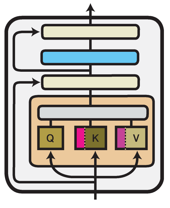
Illustration of the Prefix Tuning method within one Transformer layer. Trained components are colored in shades of magenta.
Prefix Tuning (Li and Liang, 2021) introduces new parameters in the multi-head attention blocks in each Transformer layer.
More specifically, it prepends trainable prefix vectors \(P^K\) and \(P^V\) to the keys and values of the attention head input, each of a configurable prefix length \(l\) (prefix_length attribute):
Following the original authors, the prefix vectors in \(P^K\) and \(P^V\) are not optimized directly but reparameterized via a bottleneck MLP.
This behavior is controlled via the flat attribute of the configuration.
Using PrefixTuningConfig(flat=True) will create prefix tuning vectors that are optimized without reparameterization.
Example:
from adapters import PrefixTuningConfig

config = PrefixTuningConfig(flat=False, prefix_length=30)
model.add_adapter("prefix_tuning", config=config)
As reparameterization using the bottleneck MLP is not necessary for performing inference on an already trained Prefix Tuning module, adapters includes a function to “eject” a reparameterized Prefix Tuning into a flat one:
model.eject_prefix_tuning("prefix_tuning")
This will only retain the necessary parameters and reduces the size of the trained Prefix Tuning.
Papers:
Prefix-Tuning: Optimizing Continuous Prompts for Generation (Li and Liang, 2021)
Compacter
Configuration class: CompacterConfig, CompacterPlusPlusConfig
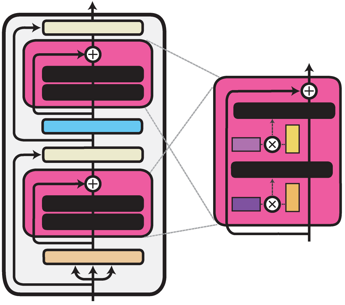
Illustration of the Compacter method within one Transformer layer. Trained components are colored in shades of magenta.
The Compacter architecture proposed by Mahabadi et al., 2021
is similar to the bottleneck adapter architecture. It only exchanges the linear down- and
up-projection with a PHM layer. Unlike the linear layer, the PHM layer constructs its weight matrix from two smaller matrices, which reduces the number of parameters.
These matrices can be factorized and shared between all adapter layers. You can exchange the down- and up-projection layers from any of the bottleneck adapters described in the previous section
for a PHM layer by specifying use_phm=True in the config.
The PHM layer has the following additional properties: phm_dim, shared_phm_rule, factorized_phm_rule, learn_phm,
factorized_phm_W, shared_W_phm, phm_c_init, phm_init_range, hypercomplex_nonlinearity
For more information, check out the BnConfig class.
To add a Compacter to your model, you can use the predefined configs:
from adapters import CompacterConfig

config = CompacterConfig()
model.add_adapter("dummy", config=config)
Papers:
COMPACTER: Efficient Low-Rank Hypercomplex Adapter Layers (Mahabadi, Henderson and Ruder, 2021)
LoRA
Configuration class: LoRAConfig
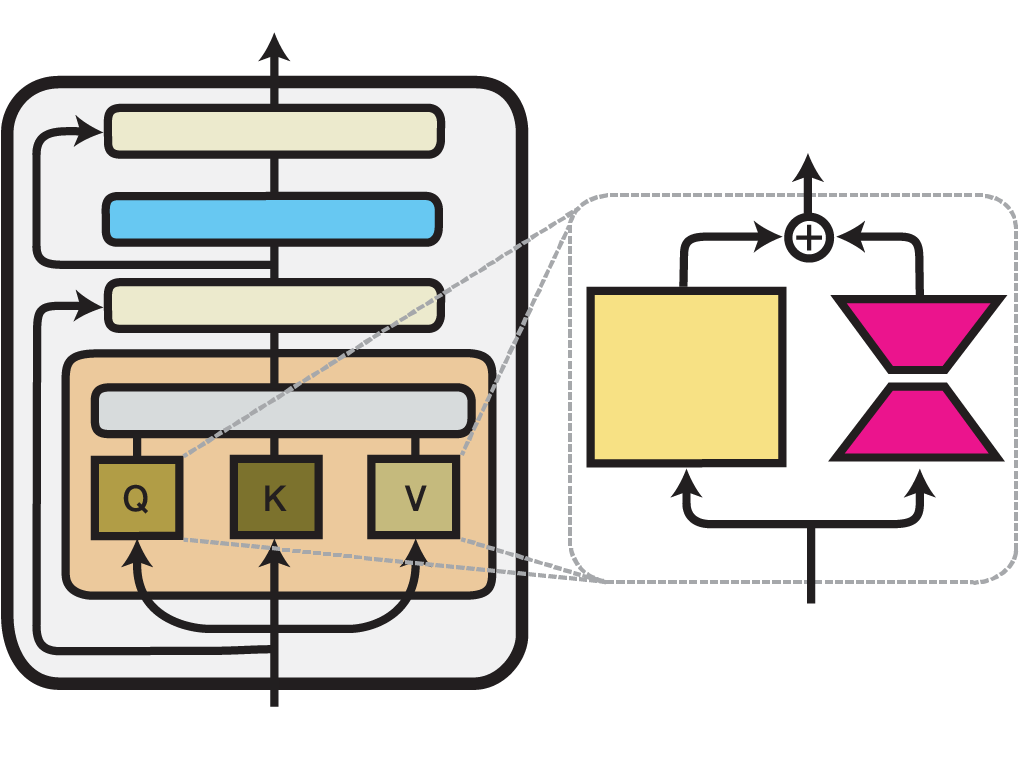
Illustration of the LoRA method within one Transformer layer. Trained components are colored in shades of magenta.
Low-Rank Adaptation (LoRA) is an efficient fine-tuning technique proposed by Hu et al. (2021). LoRA injects trainable low-rank decomposition matrices into the layers of a pre-trained model. For any model layer expressed as a matrix multiplication of the form \(h = W_0 x\), it performs a reparameterization, such that:
Here, \(A \in \mathbb{R}^{r\times k}\) and \(B \in \mathbb{R}^{d\times r}\) are the decomposition matrices and \(r\), the low-dimensional rank of the decomposition, is the most important hyperparameter.
While, in principle, this reparameterization can be applied to any weight matrix in a model, the original paper only adapts the attention weights of the Transformer self-attention sub-layer with LoRA.
adapters additionally allows injecting LoRA into the dense feed-forward layers in the intermediate and output components of a Transformer block.
You can configure the locations where LoRA weights should be injected using the attributes in the LoRAConfig class.
Example:
from adapters import LoRAConfig

config = LoRAConfig(r=8, alpha=16)
model.add_adapter("lora_adapter", config=config)
In the design of LoRA, Hu et al. (2021) also pay special attention to keeping the inference latency overhead compared to full fine-tuning at a minimum.
To accomplish this, the LoRA reparameterization can be merged with the original pre-trained weights of a model for inference.
Thus, the adapted weights are directly used in every forward pass without passing activations through an additional module.
In adapters, this can be realized using the built-in merge_adapter() method:
model.merge_adapter("lora_adapter")
To continue training on this LoRA adapter or to deactivate it entirely, the merged weights first have to be reset again:
model.reset_adapter()
Papers:
LoRA: Low-Rank Adaptation of Large Language Models (Hu et al., 2021)
(IA)^3
Configuration class: IA3Config
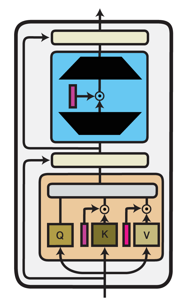
Illustration of the (IA)^3 method within one Transformer layer. Trained components are colored in shades of magenta.
Infused Adapter by Inhibiting and Amplifying Inner Activations ((IA)^3) is an efficient fine-tuning method proposed within the T-Few fine-tuning approach by Liu et al. (2022). (IA)^3 introduces trainable vectors \(l_W\) into different components of a Transformer model, which perform element-wise rescaling of inner model activations. For any model layer expressed as a matrix multiplication of the form \(h = W x\), it therefore performs an element-wise multiplication with \(l_W\), such that:
Here, \(\odot\) denotes element-wise multiplication where the entries of \(l_W\) are broadcasted to the shape of \(W\).
Example:
from adapters import IA3Config

config = IA3Config()
model.add_adapter("ia3_adapter", config=config)
The implementation of (IA)^3, as well as the IA3Config class, are derived from the implementation of LoRA, with a few main modifications.
First, (IA)^3 uses multiplicative composition of weights instead of additive composition, as in LoRA.
Second, the added weights are not further decomposed into low-rank matrices.
These modifications are controlled via the composition_mode configuration attribute by setting composition_mode="scale".
Additionally, as the added weights are already of rank 1, r=1 is set.
Beyond that, both methods share the same configuration attributes that allow you to specify in which Transformer components rescaling vectors will be injected.
Following the original implementation, IA3Config adds rescaling vectors to the self-attention weights (selfattn_lora=True) and the final feed-forward layer (output_lora=True).
Further, you can modify which matrices of the attention mechanism to rescale by leveraging the attn_matrices attribute.
By default, (IA)^3 injects weights into the key (‘k’) and value (‘v’) matrices but not in the query (‘q’) matrix.
Finally, similar to LoRA, (IA)^3 also allows merging the injected parameters with the original weight matrices of the Transformer model. E.g.:
# Merge (IA)^3 adapter
model.merge_adapter("ia3_adapter")

# Reset merged weights
model.reset_adapter()
Papers:
Vera
Vera is a LoRA based fine-tuning method proposed by Kopiczko et al. (2024). In Vera, we add frozen matrices A and B that are shared across all layers. It reduces the number of trainable parameters but maintains the same performance when compared to LoRA. Furthermore, trainable scaling vectors \(b\) and \(d\) are introduced and are multipled by the frozen matrices to result in the equation:
where \Lambda_{b} and \Lambda_{d} receive updates during training.
Example:
from adapters import VeraConfig

config = VeraConfig()
model.add_adapter("vera_config", config=config)
Using the VeraConfig, you can specify the initialization of the scaling vectors and the Vera initialization of frozen weights B and A via the parameter init_weights.
Papers:
VeRA: Vector-based Random Matrix Adaptation (Kopiczko et al., 2024)
DoRA
DoRA refers to Weight-Decomposed Low-Rank Adaptation, and is a LoRA based fine-tuning method proposed by Liu et al. (2024). Using the DoRA method, we decompose the pre-trained weights W_{0} into a magnitude \(m\) and directional \(d\) and fine-tunes both. The magnitude component \(m\) is a vector while the \(d\) directional component is a matrix that is uses LoRA matrices \(B\) and \(A\). Furthermore, we keep the columns of the directional component unit vectors by dividing the matrix by its norm. During training, we calculate the hidden_states using both the magnitude component and directional component via the equation:
.. note::
the DoRA Method can work in tangent with both LoRA and Vera. You can utilize DoRA with LoRA either by using the DoRAConfig or by using a LoRAConfig with the use_dora parameter set to True. Similarly, the DvoRAConfig is a a shortcut for the VeraConfig that utilizes DoRA via the use_dora parameter.
_Example_:
```python
config = DoRAConfig()
model.add_adapter("dora_adapter", config=config)
Papers:
DoRA: Weight-Decomposed Low-Rank Adaptation (Liu et al., 2024)
Prompt Tuning
Prompt Tuning is an efficient fine-tuning technique proposed by Lester et al. (2021). Prompt tuning adds tunable tokens, called soft-prompts, that are prepended to the input text. First, the input sequence \({x_1, x_2, \dots, x_n }\) gets embedded, resulting in the matrix \(X_e \in \mathbb{R}^{n \times e}\) where \(e\) is the dimension of the embedding space. The soft-prompts with length \(p\) are represented as \(P_e \in \mathbb{R}^{p \times e}\). \(P_e\) and \(X_e\) get concatenated, forming the input of the following encoder or decoder:
The PromptTuningConfig has the properties:
prompt_length: to set the soft-prompts length \(p\)prompt_init: to set the weight initialisation method, which is either “random_uniform” or “from_string” to initialize each prompt token with an embedding drawn from the model’s vocabulary.prompt_init_textas the text use for initialisation ifprompt_init="from_string"
combine: To define if the prefix should be added before the embedded input sequence or after the BOS token
To add Prompt Tuning to your model, you can use the predefined configs:
from adapters import PromptTuningConfig

config = PromptTuningConfig(prompt_length=10)
model.add_adapter("dummy", config=config)
Papers:
The Power of Scale for Parameter-Efficient Prompt Tuning (Lester et al., 2021)
ReFT
Configuration class: ReftConfig
Representation Fine-Tuning (ReFT), as first proposed by Wu et al. (2024), leverages so-called interventions to adapt the pre-trained representations of a language model. Within the context of ReFT, these interventions can intuitively be thought of as adapter modules placed after each Transformer layer. In the general form, an intervention function \(\Phi\) can thus be defined as follows:
Here, \(R \in \mathbb{R}^{r \times d}\) and \(W \in \mathbb{R}^{r \times d}\) are low-rank matrices of rank \(r\). \(h\) is the layer output hidden state at a single sequence position, i.e. interventions can be applied independently at each position.
Based on this general form, the ReFT paper proposes multiple instantiations of ReFT methods supported by Adapters:
LoReFT enforces orthogonality of rows in \(R\). Defined via
LoReftConfigor via theorthogonalityattribute as in the following example:
config = ReftConfig(
    layers="all", prefix_positions=3, suffix_positions=0, r=1, orthogonality=True
)  # equivalent to LoreftConfig()
NoReFT does not enforce orthogonality in \(R\). Defined via
NoReftConfigor equivalently:
config = ReftConfig(
    layers="all", prefix_positions=3, suffix_positions=0, r=1, orthogonality=False
)  # equivalent to NoreftConfig()
DiReFT does not enforce orthogonality in \(R\) and additionally removes subtraction of \(R h\) in the intervention, Defined via
DiReftConfigor equivalently:
config = ReftConfig(
    layers="all", prefix_positions=3, suffix_positions=0, r=1, orthogonality=False, subtract_projection=False
)  # equivalent to DireftConfig()
In addition, Adapters supports configuring multiple hyperparameters tuned in the ReFT paper in ReftConfig, including:
prefix_positions: number of prefix positionssuffix_positions: number of suffix positionslayers: The layers to intervene on. This can either be"all"or a list of layer idstied_weights: whether to tie parameters between prefixes and suffixes
Papers:
ReFT: Representation Finetuning for Language Models (Wu et al., 2024)